Notes

The five coordinate spaces a vertex passes through between the scene and the screen, and the exact matrix or formula that moves it each direction. Ordered here to match the actual rendering pipeline: World → Camera → Clip → Screen → Pixel.

The five spaces, in rendering order

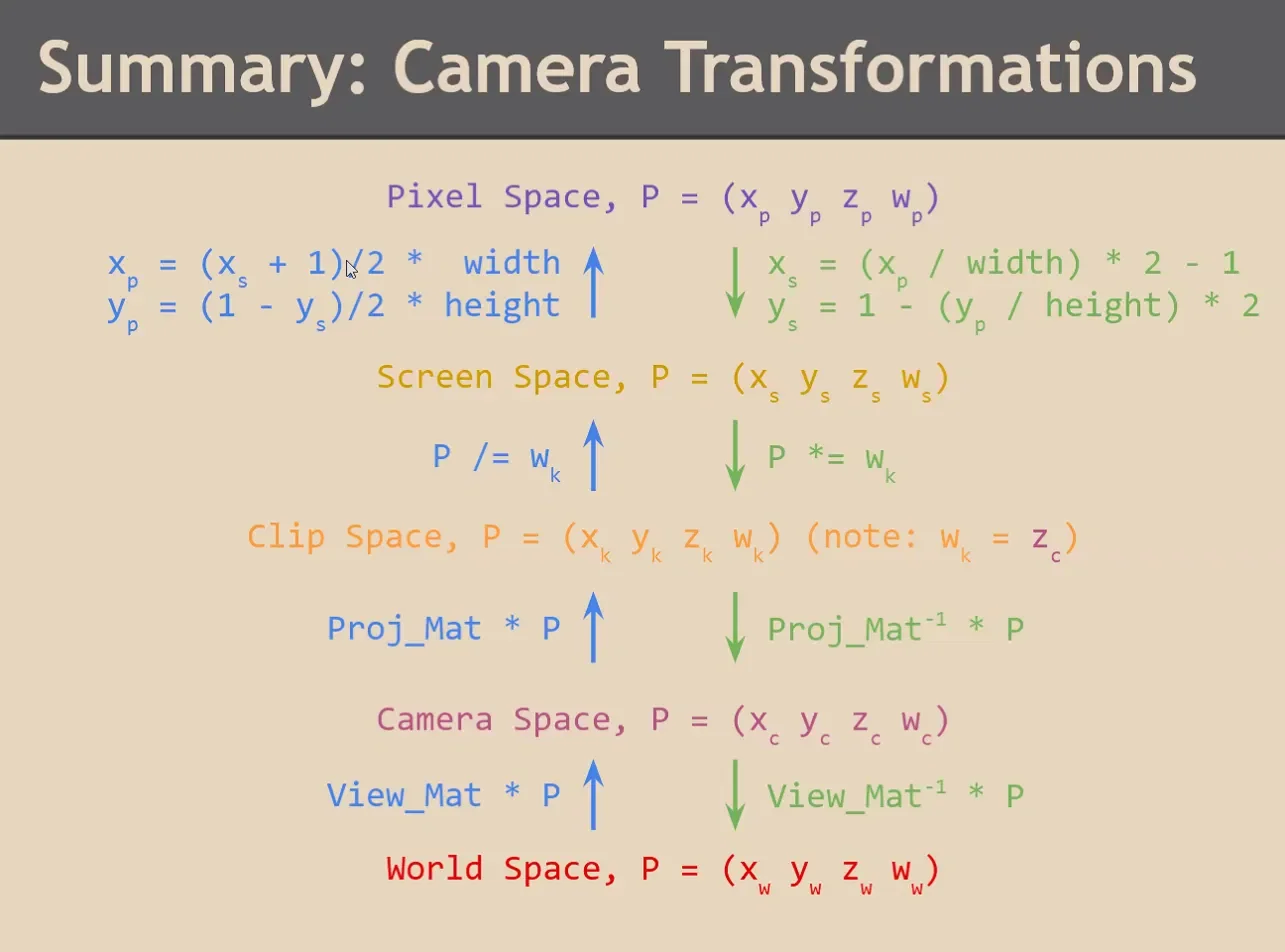
Step 1: World → Camera Space

View_Mat * P — the camera’s own world transform, inverted, so that after this the camera sits at the origin looking down a fixed axis. Reverse: View_Mat⁻¹ * P.

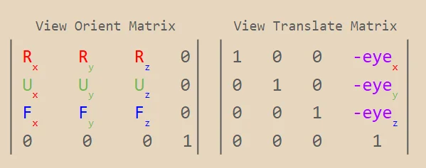
Why the order is Rᵀ * T⁻¹: the view matrix moves the world, not the camera. Placing the camera in the world is T * R; the view matrix undoes that, and inverting a product reverses the order:

$$V = (TR)^{-1} = R^{-1}T^{-1} = R^{T}T^{-1}$$

So orientation ends up on the left. R is orthonormal, so R⁻¹ = Rᵀ — just write the camera axes as rows instead of columns. Multiplied out, the fourth column is -dot(axis, eye), not -eye, because the translation is expressed in the camera axes. See Matrix composition order (SRT) for the right-to-left rule this inverts.

Step 2: Camera → Clip Space

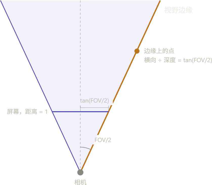
Proj_Mat * P — encodes the field of view and near/far planes, and sets up $w_k = z_c$ (clip-space w is just a copy of camera-space depth, carried along purely so the next step has something to divide by). Reverse: Proj_Mat⁻¹ * P. 透视矩阵其实是为了下一步透视除法做准备，他定义了我们眼前的视锥体，check pic2 below.

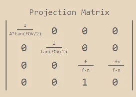
### What each row does Each row produces one output component. Read them independently.

Rows 1 and 2: fit the field of view to the screen. $x' = \frac{S}{A}x$, $y' = Sy$, with $S = 1/\tan(FOV/2)$.

After the divide, a point sitting exactly on the edge of the view has lateral offset over depth equal to $\tan(FOV/2)$, the same ratio for every point on that edge line. So without scaling, the visible region after the divide is $[-\tan(FOV/2), \tan(FOV/2)]$, which changes with FOV. Multiplying by $S$ pulls that edge to exactly $\pm1$, so whatever you can see fills NDC’s $[-1, 1]$ and the viewport transform can treat every camera the same way.

Narrow FOV means small $\tan$, big $S$, everything magnified. That’s zooming in.

$A$ = width / height. FOV is vertical. On a wide screen, NDC’s $[-1,1]$ is spread over more pixels horizontally than vertically, so one NDC unit is physically longer in x. Dividing x by $A$ cancels that stretch; skip it and circles render as ellipses. With a square screen $A = 1$ and it does nothing, which is why a bug here hides until the window isn’t square.

Row 3: prepare depth. $z' = Pz + Q$. After the divide this becomes $P + Q/z$. $P$ and $Q$ are the solution to two conditions, near plane lands on 0 and far plane lands on 1:

$$P + \frac{Q}{n} = 0, \qquad P + \frac{Q}{f} = 1 \quad\Rightarrow\quad P = \frac{f}{f-n},\quad Q = \frac{-fn}{f-n}$$

Without $Q$, every point would come out as $z/z = 1$ and the depth buffer would have nothing to compare. $P + Q/z$ is not linear in $z$: with $n = 1, f = 100$, the first half of the range already uses up 0 to 0.99. Precision piles up near the camera, which is why a tiny near plane causes z-fighting in the distance.

Row 4: park the divisor. $(0, 0, 1, 0)$ copies camera-space $z$ into $w$. A matrix can only multiply and add, it can’t divide, so it stores the number the next step needs to divide by. An ordinary transform has $(0,0,0,1)$ here and keeps $w = 1$; moving that 1 one column left is the entire trick.

In glm (column-major) this is glm::vec4(0, 0, P, 1) passed as the third column: the 1 lands at m[2][3], which is row 4, column 3.

Worked example

FOV 45°, $A = 1$, $n = 1$, $f = 100$ gives $S \approx 2.414$, $P \approx 1.0101$, $Q \approx -1.0101$.

Camera-space point	After matrix $(x', y', z', w')$	After $\div w'$ (NDC)
$(2, 1, 5, 1)$	$(4.828,\ 2.414,\ 4.040,\ 5)$	$(0.966,\ 0.483,\ 0.808)$
$(2, 1, 10, 1)$	$(4.828,\ 2.414,\ 9.091,\ 10)$	$(0.483,\ 0.241,\ 0.909)$

Same lateral position, twice the depth. After the matrix, $x'$ and $y'$ are identical; only $w'$ differs. After the divide, the far point is half the size. The matrix sets things up, the divide is what makes far things small.

Sign-convention note: some derivations write $w_c = -z_v$ instead (right-handed view space, camera looking down $-z$, so visible points have negative $z_v$ and the negation keeps $w$ positive). Whether you need the negative sign depends on how your source already defines $z_c$ — check before assuming one form is wrong. See Clipping for where this actually comes from in the projection matrix.

Between this step and the next, clipping happens — triangles are cut against the frustum boundaries while still in clip space, before anything is divided. See Clipping for why this order is mandatory, not just convention.

Step 3: Clip → Screen Space (perspective divide)

$$P_{screen} = P_{clip} / w_k$$

The step that actually creates the perspective effect. Reverse: P *= wk. See Perspective-correct interpolation for why this divide distorts linearity in screen space, and how rasterization corrects for it when interpolating attributes. 透视除法只是想象把一个视锥体变成一个高度和宽度在[-1, 1]，深度[0, 1]的盒子。

Step 4: Screen → Pixel Space (viewport transform)

$$x_p = \frac{x_s + 1}{2} \times \text{width}, \qquad y_p = \frac{1 - y_s}{2} \times \text{height}$$

Reverse:

$$x_s = \frac{x_p}{\text{width}} \times 2 - 1, \qquad y_s = 1 - \frac{y_p}{\text{height}} \times 2$$

Why y flips here: NDC’s y increases upward (math convention), pixel space’s y increases downward (row 0 is the top of the screen) — this is the one step where that flip is actually applied.

Gotcha

Rasterization (both coverage-test methods) operates in pixel space — the final destination of this whole pipeline, it needs actual pixel coordinates to compare against. But the w value from before the perspective divide (Step 3) has to be preserved and carried through anyway, because attribute interpolation (perspective-correct interpolation) needs it even though the coverage test itself doesn’t.

Related

Perspective-correct interpolation
Rasterization
Clipping